Reading & writing Excel files (Microsoft Graph)

This tutorial shows how to read from and write to an Excel file using Microsoft Graph in a workflow, based on a concrete example: exporting GRC (Governance, Risk & Compliance) contract analysis results into a structured Excel report.

Example scenario

You have a workflow that produces a structured analysis result (e.g., a “thematic gap matrix” with domains, severity, regulatory references, and remediation suggestions). The goal is to generate an Excel report that stakeholders can review, share, and archive.

In this guide, we’ll:

• Prepare an Excel template that the workflow can reliably write into
• Define the data model and map your workflow output to report columns
• Transform your JSON output into the 2D array format required by Microsoft Graph
• Read the workbook and target the right worksheet
• Create an Excel table (once per workbook) and append rows to it (repeatedly)
• Validate the generated Excel report (and optionally read it back)

Step 1 — Prepare your Excel template

Start by creating an Excel file that will act as the report template.

The template should contain:

• A title row (optional)
• A header row with the column names you want in your report
• A hidden “placeholder” row right under the header row (important)

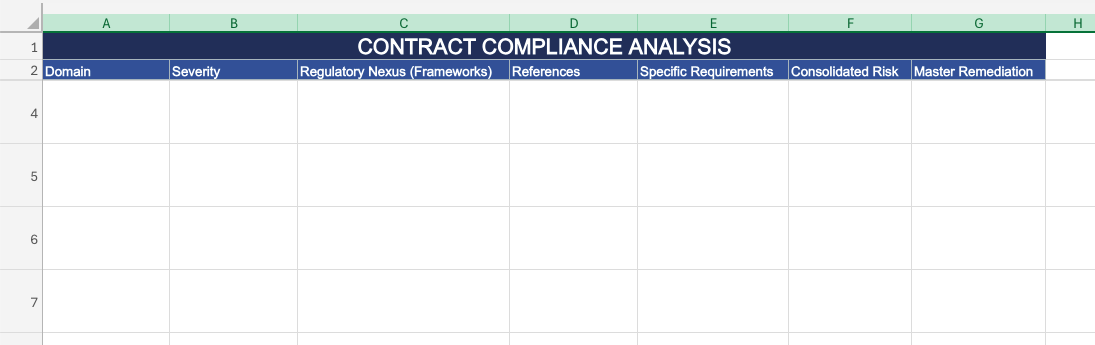
In our example template, the report is called “Contract Compliance Analysis”, and the header row contains the following columns:

• Domain
• Severity
• Regulatory Nexus (Frameworks)
• References
• Specific Requirements
• Consolidated Risk
• Master Remediation

Add the hidden placeholder row

Insert one empty row directly under the header row (i.e., the first data row) and hide it.

With the template above:

• Row 2 contains the headers (Domain, Severity, …)
• Row 3 should be an empty row that you hide

Why this hidden row matters:

• Many Excel “write rows” operations in Graph work best when you write into an existing Table.

• Creating a Table requires the range to include at least one data row.

• The hidden row acts as the initial data row so you can convert the header + placeholder into a Table, without visually polluting the report.

  

Step 2 — Define the data you want to print

Assume your workflow output contains a list of rows under thematic_gap_matrix, where each item represents one “domain analysis” line to export.

What the raw AI output looks like (before formatting)

In this example, the raw JSON is generated by an AI··Task step in the workflow, and includes thematic_gap_matrix plus other computed fields.

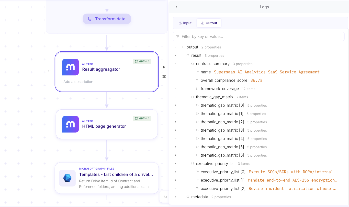
For the Excel template above, we assume each item contains the following fields (you can rename to match your own output):

• domain
• impact_severity
• regulatory_nexus.framework (array)
• regulatory_nexus.reference (array)
• regulatory_nexus.specific_requirement (array)
• consolidated_risk
• master_remediation

At export time, each Excel row should map to:

1. Domain → domain
2. Severity → impact_severity
3. Regulatory Nexus (Frameworks) → join regulatory_nexus.framework
4. References → join regulatory_nexus.reference
5. Specific Requirements → join regulatory_nexus.specific_requirement
6. Consolidated Risk → consolidated_risk
7. Master Remediation → master_remediation

Step 3 — Format data for writing to Excel via Microsoft Graph

Most Microsoft Graph Excel write operations expect tabular data as a 2D array (rows × columns).

The core rule: always send a 2D array

• One row still needs the shape [[...]].
• Multiple rows use [[...], [...], ...].

Columns must match your Excel table or range

Each inner array is a row, and its items must be in the exact same order as the Excel columns. If your table has 7 columns, each row array must have 7 items.

Typical payload shape

Depending on the specific Graph endpoint/connector, the body usually includes something like:

• values: the 2D array of rows to write

Example (2 rows × 3 columns):

• values:
  • [“Value 1”, “Value 2”, “Value 3”]
  • [“Value 4”, “Value 5”, “Value 6”]

Practical formatting tips

• Convert complex fields (arrays, objects) into strings before writing (for example, join arrays with ", ").
• Keep types consistent per column when possible (numbers as numbers, dates in the format your workbook expects).
• Validate the output is strictly a list of lists before sending it to Graph.

Step 4 — Transform JSON output into Excel rows (JSONata example)

Now let’s apply those formatting rules to our concrete example data: your workflow output is usually a list of objects, but Graph expects a 2D array of row values.

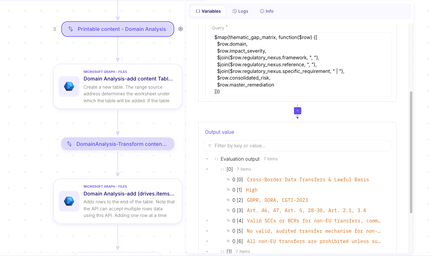
A common approach is to use a data transformation step (e.g., JSONata) to build the values payload.

The key points:

• Iterate over thematic_gap_matrix
• Output an array of rows
• Each row must be an array of values, in the exact same order as the Excel columns
• Join array fields (frameworks, references, requirements) into readable strings

Example JSONata pattern (as shown below):

• Map each item to [domain, severity, frameworks_joined, references_joined, requirements_joined, consolidated_risk, master_remediation]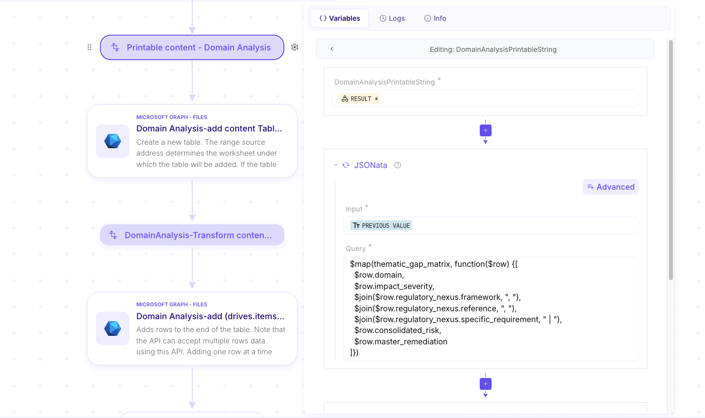

  

And you can validate the result by checking the output preview: it should be a list of row arrays (one row array per exported line).

Step 5 — Read the workbook and target the right worksheet

To write to an Excel workbook with Microsoft Graph, you first need to identify the file and retrieve workbook metadata so you can target the correct worksheet (and later, the table) for your write operations.

In this guide, we’ll assume you already have the Drive id and Drive item id for the workbook you want to write to.

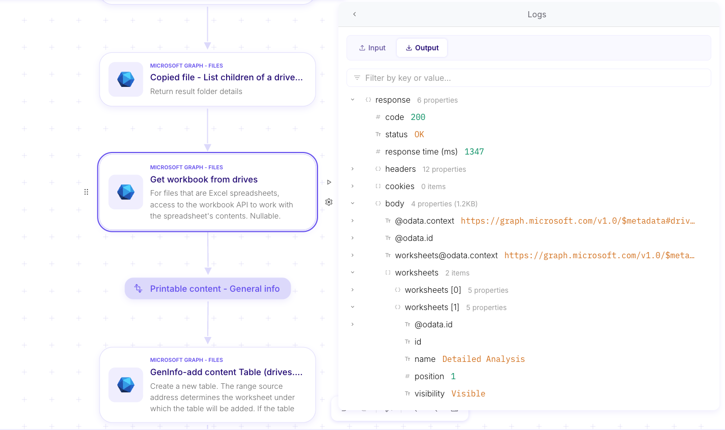
Step 5.1 — Get workbook metadata (list worksheets)

Mindflow step: Microsoft Graph - Files → “Get workbook from drives (drives.items.workbook…)”

This step retrieves the workbook metadata (including the list of worksheets) so you can select the right worksheet for downstream steps.

Inputs (what to fill)

• Drive id
• Drive item id

Output (what to look for)

• The list of worksheets (names and ids). You’ll use this output to pick the worksheet you want to write into (for example, “Detailed Analysis”).

In the example below, the workbook contains a worksheet named “Detailed Analysis”, which is the one we’ll write into.

Step 6 — Write into Excel (end-to-end outline)

A typical workflow pattern is:

1. Create the Excel table from the hidden placeholder row (once per worksheet)
2. Add rows to the table using the Graph “add rows” operation, passing the 2D values

Below are the two main steps in detail (plus a small note on retrieving and URL-encoding the Table ID between them).

---

Step 6.1 — Create the Excel table (once per workbook)

Mindflow step: Microsoft Graph - Files → “Add content table”

This is the step that converts a worksheet range into an Excel Table object. After the table exists, you will append rows to it.

Inputs (what to fill)

• Drive id
  • The document library where the workbook lives.
• Drive item id
  • The workbook file identifier.
• Address
  • The worksheet + cell range to turn into a Table.
  • Format: 'Sheet name'! plus the cell range (for example, 'Detailed Analysis'!A3:G3)
  • The sheet name must be wrapped in single quotes.
  • The range should start at the hidden placeholder row you created (the first data row), so the table contains headers + at least one data row.
  • Example: 'Detailed Analysis'!A3:G3
    • Here A3:G3 targets the hidden row (Row 3) under the headers.
• Has headers
  • Enable this so Graph treats the row above your range as column headers.

Example screenshots (sensitive data obfuscated)

• Screenshot 1 — Add content table (input): shows the Drive id, Drive item id, and Address set to 'Sheet name'!A3:G3.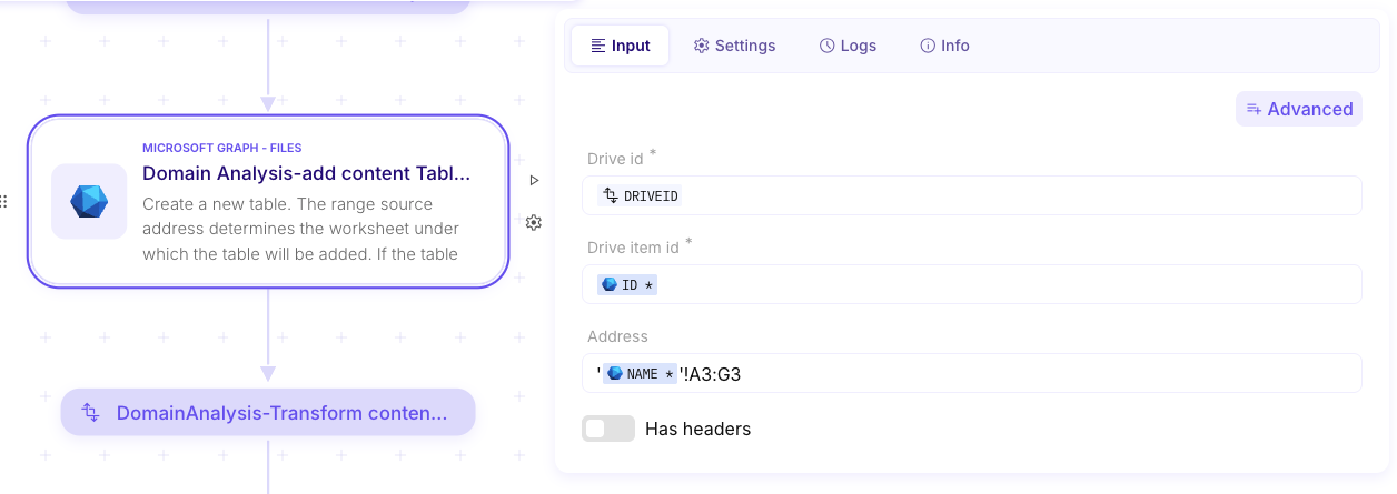

  

Step 6.2 — Retrieve and URL-encode the Table ID

After the table is created, the output contains the table identifier.

Output (what to look for)

• In the response body, find the table id (this is the workbook table id you’ll use for row insertion).

Example screenshots (sensitive data obfuscated)

• Screenshot 2 — Add content table (output): highlights the returned table id.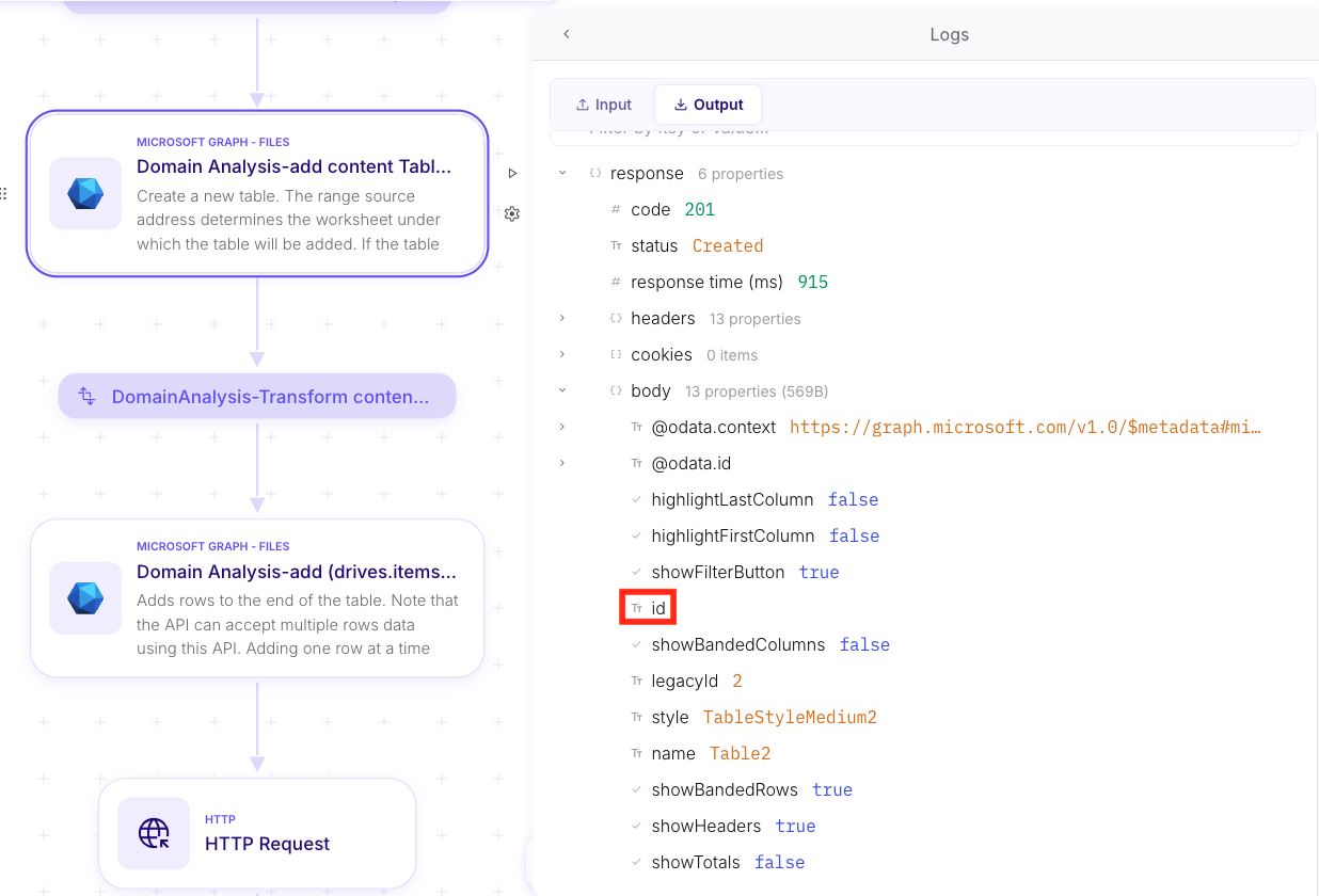

  

Some Graph operations require this table id to be URL encoded when passed downstream. A safe pattern is to URL-encode it systematically.

Example screenshots (sensitive data obfuscated) (2)

• Screenshot 3 — URL encode (variable transform): shows URL encoding applied to the table id output.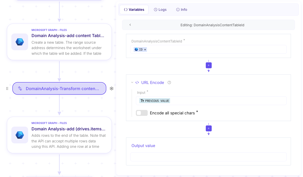

  

Step 6.3 — Add rows to the table

Mindflow step: Microsoft Graph - Files → “Add rows”

This is where you write the content into the workbook by appending row values to the table.

Inputs (what to fill)

• Drive id
• Drive item id
• Workbook table id
  • Use the (URL-encoded) table id from Step 6.2.
• Values
  • Use the transformed 2D array from the JSONata step.
  • Reminder: the shape must be [[...], [...]] (array of row arrays).

Example screenshots (sensitive data obfuscated)

• Screenshot 4 — Add rows (input): shows the Workbook table id and the Values variable passed into the step.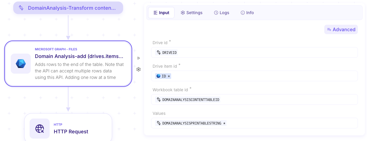

  

• Screenshot 5 — Add rows (output): shows a successful insertion and echoes back the inserted values[0].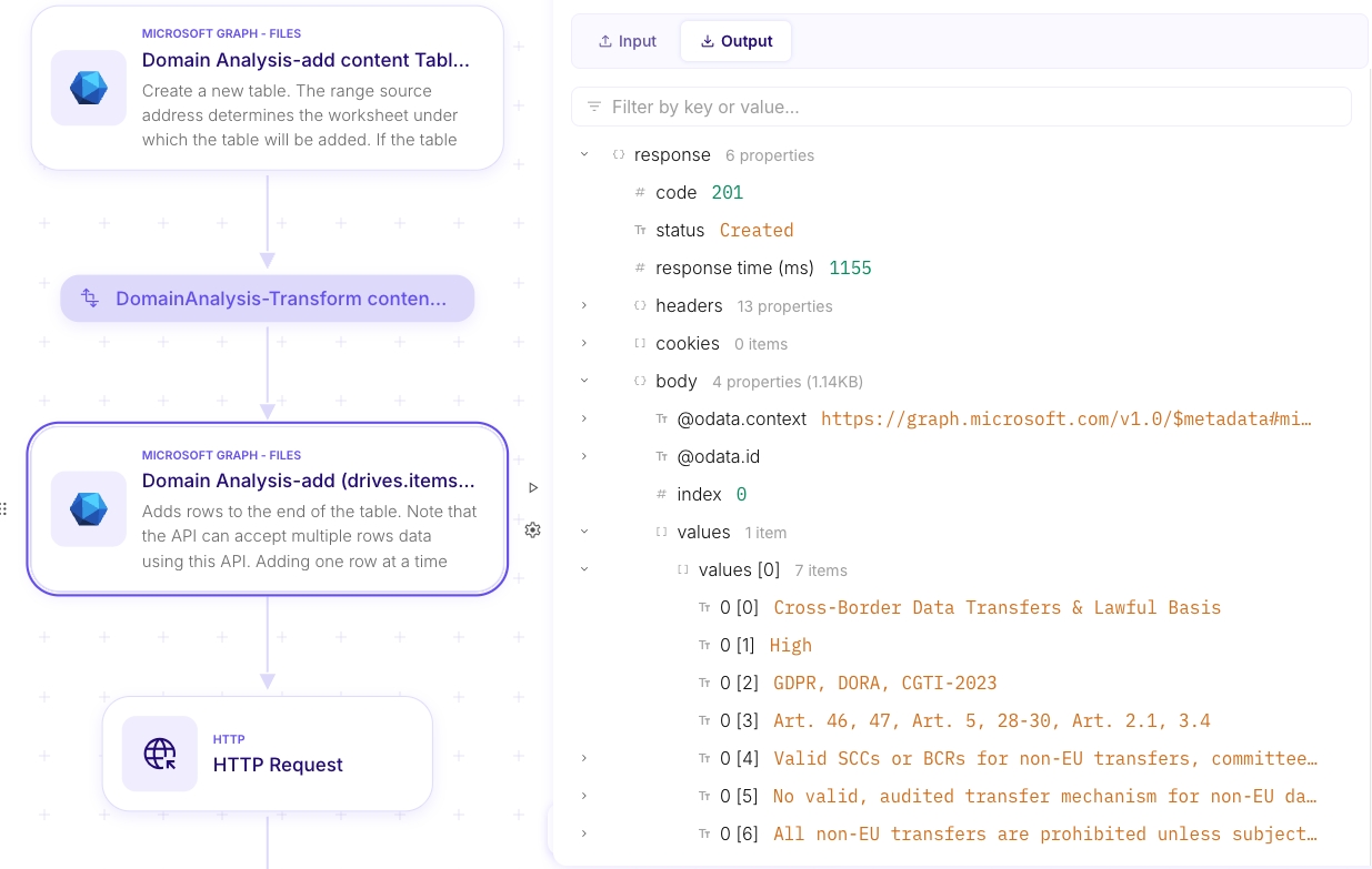

  

---

---

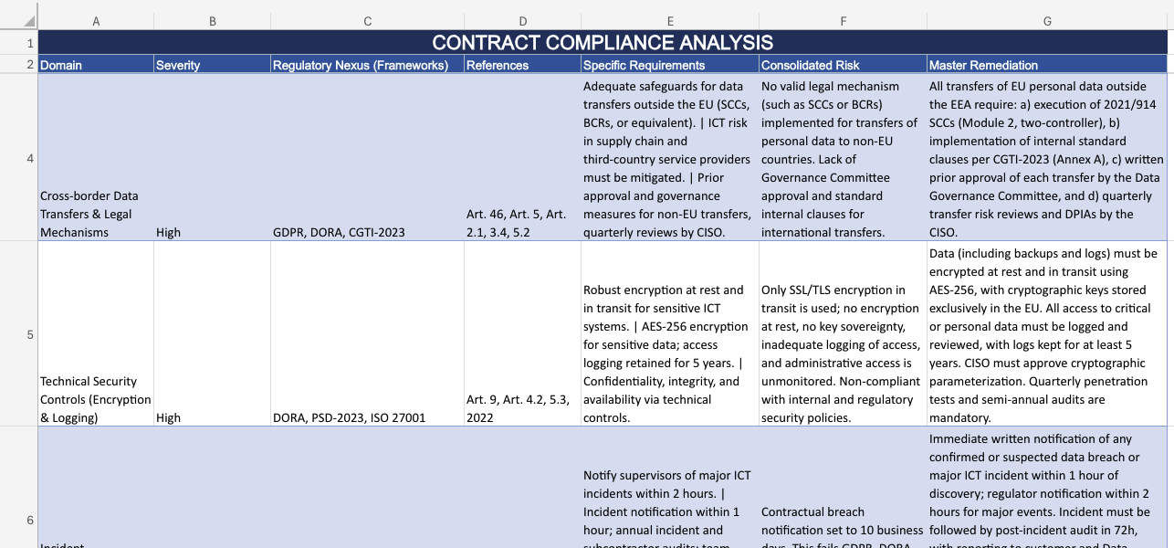
Step 7 — Validate the generated Excel report (output)

Once rows are inserted into the table, the worksheet is populated and formatted like a standard Excel report.

Example screenshots (sensitive data obfuscated)

• Screenshot — Final Excel output: shows the generated report with rows filled under the “Contract Compliance Analysis” headers.

  

---

Step 8 — Read from an Excel file (use the report you just generated)

You can also take advantage of the Excel report you just created to demonstrate how to read an Excel file back, which is useful for other use cases where an Excel workbook is an input you need to process.

The most straightforward approach is to read the worksheet’s used range.

Step 8.1 — Read worksheet content using UsedRange

Mindflow step: Microsoft Graph - Files → “UsedRange (drives.items.workbook…)”

This step returns the values found in the worksheet’s used range.

Inputs (what to fill)

• Drive id
  • The document library where the workbook lives.
• Drive item id
  • The workbook file identifier (use the same file you just wrote to).
• Workbook worksheet id
  • The worksheet identifier for the sheet you want to read.
  • This is typically retrieved from the workbook metadata step, then transformed/mapped to the format expected by the API.

Example screenshots (sensitive data obfuscated)

• Screenshot 1 — UsedRange (input): shows Drive id, Drive item id, and Workbook worksheet id populated.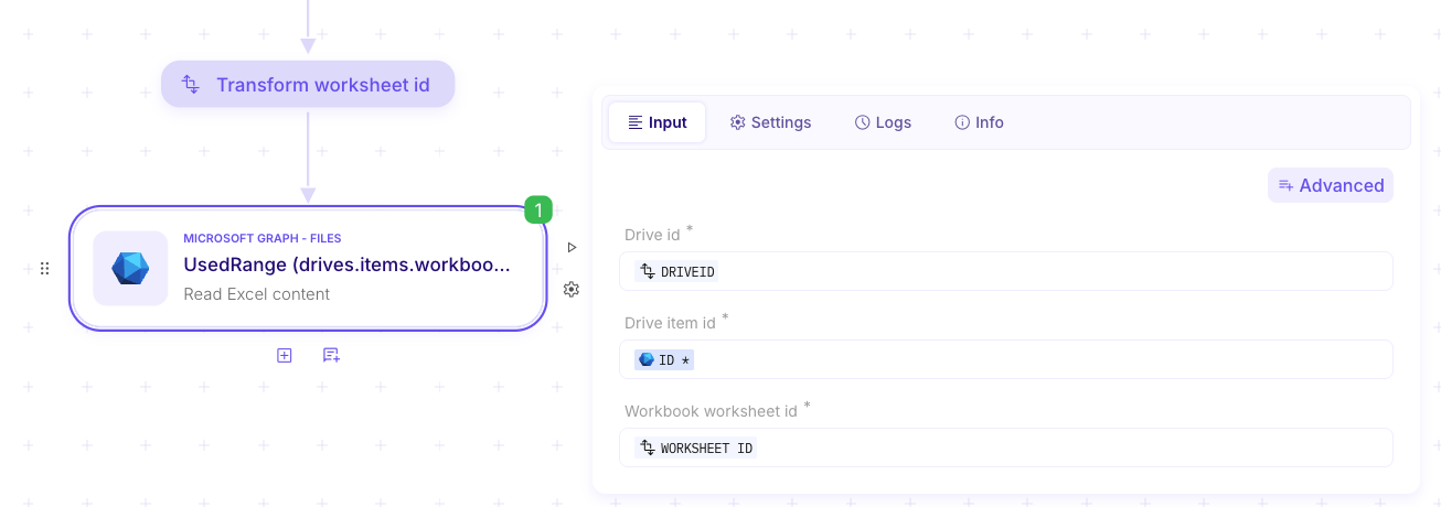

  

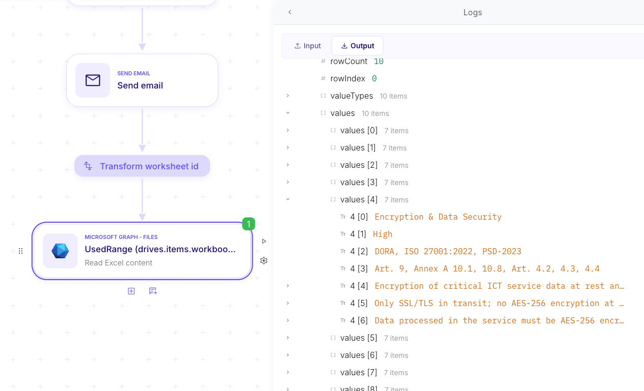
Step 8.2 — Understand the output format

The UsedRange response includes both metadata and the cell values.

Output (what to look for)

• rowCount / columnCount
  • The size of the returned range.
• values
  • A 2D array of cell values.
  • Each inner array is one row; each item in the row array is a cell value (string/number/blank).
  • This format is consistent with Graph’s general Excel representation of ranges.

Example screenshots (sensitive data obfuscated)

• Screenshot 2 — UsedRange (output): highlights rowCount and the values 2D array (rows × columns).